Stanford CS231A: Computer Vision, From 3D Reconstruction to Recognition
이 포스트는 Stanford CS231A 강의의 첫 번째 강의 노트인 “Camera Models”를 정리한 것입니다.
원본 강의 노트: 01-camera-models.pdf
1. Introduction
케마라는 computer viewion에서 가장 필수인 툴이다. 이번 포스팅에서는 이러한 computer vision에서 카메라가 어떻게 수학적으로 표현이 되어는지 이해하도록 한다.
2. Pinhole Cameras
2.1 Basic Concept
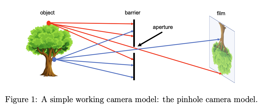
일반적인 카메라 시스템은 3D world에 있는 object를 2D로 매핑을 한다. 일반적인 카메라를 기본으로 하는 모델은 Pinhole Camera로써 접근을 한다. 이는 조리개(aperture)로 장벽을 두어서 설계가 되어져있다. 이해가 쉽게 아래의 그림에서 Figure 1에서 보는것과같이 3D object 여러개의 광선을 보내게 되는데 이경우 flim에 image가 생기지 않는다. 하지만 aperture가 있을 경우에서는 image가 생기게 되어지며 일대일 대응으로 만들수 있어진다.
2.2 Formal Construction
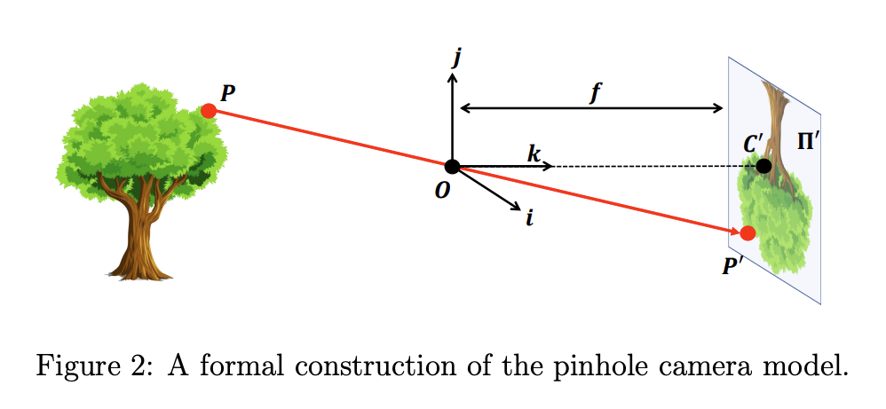
Figure 2에서 보면 pinhole camera의 구성을 보자. flim에 object가 나오는 경우를 우리가 흔히 아는 image 또는 retinal plane으로 불려진다. aperture의 경우 수식적으로 $O$으로 불리던지 center of the camera 라로 불린다. 이때 retinal plane과 $O$까지의 거리는 focal length=$f$로 불린다. 일반적으로 이미지 평면은 핀홀 뒤에 있지만, 수학적으로는 편의를 위해 이미지 평면을 카메라 앞쪽에 놓는 경우가 있다. 이 경우, 투영된 이미지가 상하·좌우 반전되지 않아서 계산이 더 단순해진다. 이때 맽히는 것은 virtual image or virtual retinal plane 라고 불린다.
2.3 Projection Equation
이제 수식적으로 보면 $P=\begin{bmatrix} x & y & z \end{bmatrix}^{T}$ 은 어떠한 3D world상의 point라고 한다. $P$는 image plane $\Pi’$에 매핑=projection이 되어지며 이는 $P’=\begin{bmatrix} x’ & y’\end{bmatrix}^{T}$로 표현이 되어진다. 마찬가지로, 핀홀 자체도 이미지 평면에 투영될 수 있으며, 그 결과 새로운 점 $C’$를 얻는다. 그렇다면 우리는 좌표계(coordinate system)을 정의하면 원점($O$)을 중심으로 하고 Figure2에 있는 $\begin{bmatrix} i & j & k \end{bmatrix}$로 정의할수 있다. 각 parameter의 경우 $k$축은 이미지 평면을 향해 수직으로 뻗는 방향, $i,j$는 이미지 평면 내에서 가로·세로 방향로 정의 되어진다.
이 부분에 대해서 햇깔릴수 있는데 쉽게 이해하기 위해서 카메라가 바라보는 방향이 $k$축이 되도록 좌표계를 잡으면 된다.
이러한 좌표계를 카메라 기준 좌표계(camera reference system) 또는 카메라 좌표계(camera coordinate system)이라고 불린다. 정리하면 $P’$는 3D point, $P$는 $\Pi’$에 투영된 point이고 원점은 $O$이다. 이 3개의 점은 $P’C’O$삼각형으로 되어지며 앞전에 $f$를 바탕을 사용하면 삼각형의 법칙을 통해서 projection이 되어진다. 아래는 수식이다.
\[P'=\begin{bmatrix} x' & y' \end{bmatrix}=\begin{bmatrix} f \frac{x}{z} & f \frac{y}{z} \end{bmatrix}\]2.4 Aperture Size Effects
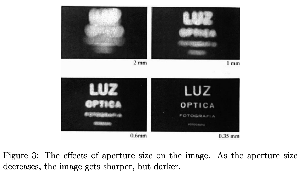
Camera모델의 경우 아래의 이미지에서 보이는 듯이 aperture의 size에 따라서 이미지가 바뀐다. 작으면 선명해지지만 빛의 양이 줄어들어서 유실될수도 있고 커지면 오히려 흐릿해진다. 그렇다면 빛을 전부 받으면서 밝게 이미지를 유지할수 있는 방법이 없는지 생각하게 되어지는데 이때 렌즈(Lenses)의 개념이 나오게 되어진다.
3. Cameras and Lenses
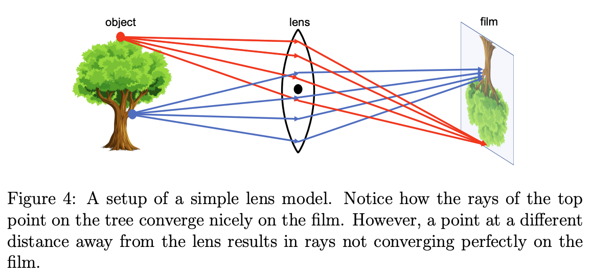
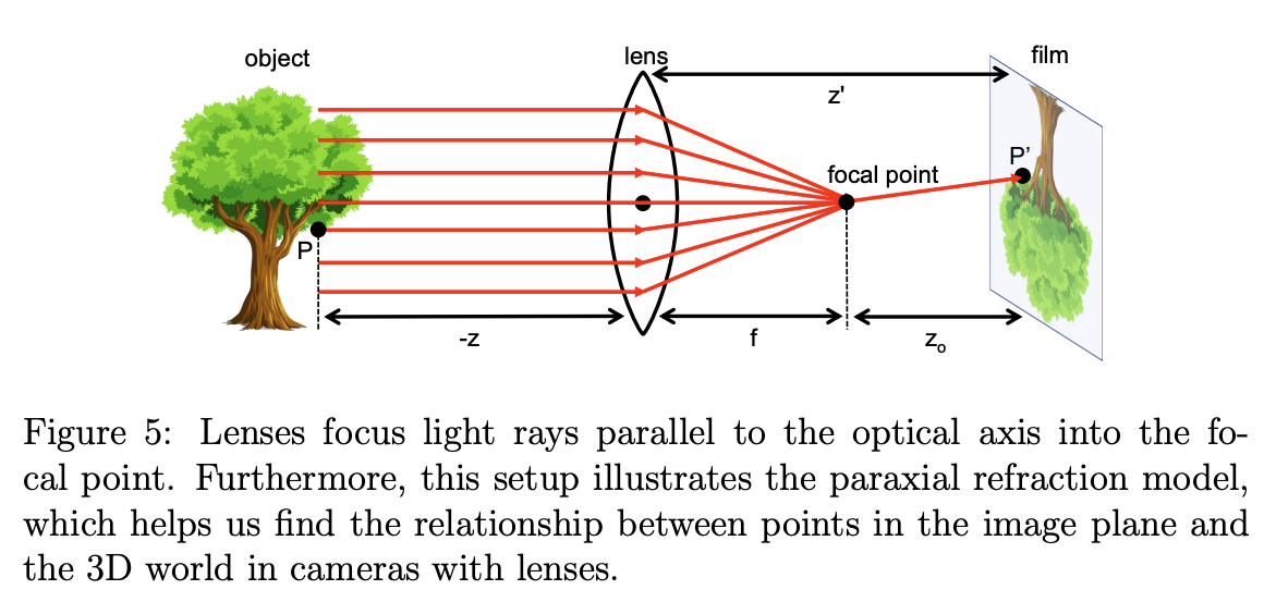
렌즈를 사용하게 되어지면 선명도(crispness)와 밝기(brightness)에 대해서 완화할수 있다. 아래의 그림처럼 $P$에서 나오는 모든 빛들은 굴절되어저 $P’$로 모이게 되어진다. 하지만 모든 3D point에 되는것이 아니라 특정 $P$에 대해서망 성립을 한다. 단순하게 생각해보면 쉽다. image plane으로 부터 $P$보다 먼 위치에 있는 점 $Q$가 있다고 가정했으면 이는 렌즈에 초점 거리가 맡지 않아서 흐릭하게 찍히게 되어진다. 카메라에서는 이러한 심도(depth of field)라는 개념인데 결국 선명한 사진을 찍을수 있는 위치가 필요한다.
3.1 Focal Point and Paraxial Refraction Model
Figure 5에서 보면 focal point라고 불리는 한점에 보이게 되어진다. 렌즈의 개념이 나오게 되어지면 $f$는 랜즈의 중심과 focal point까지의 거리로 정의한다. 이때 $P’$로 되어지는건 이전의 수식과 달라지는데 image plane과 렌즈의 거리를 $z’$가 있음으로 아래의 삼각형의 법칙으로 아래와 같은 수식으로 표현이 되어진다. 처음은 왜 이런지 이해가 안됬지만 기본적으로 광선은 직진한다고 가정하기 때문에 pinhole모델과 같은 거의 투영식을 만족함. 근사적으로 거의 같음.
\[P'=\begin{bmatrix} x' \\ y' \end{bmatrix}=\begin{bmatrix} z' \frac{x}{z} \\ z' \frac{y}{z} \end{bmatrix}\]수식으로 보았을때는 똑같이 보이지만 랜즈에서는 $z’=f+z_{0}$, 일반적은 수식은 $z’=f$이 들어가있다.
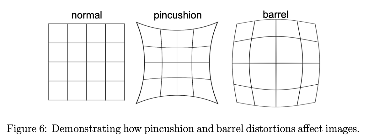
이러한 근사모델은 결국 오차가 생기게 되어지며, 및이 다양한 각도로 들어기 때문에 왜곡이 생기게 되어진다. Figure 6에서 보는것과 같이 핀쿠션 왜곡(pincushion distortion), 배럴 왜곡(barrel distortion) 이 생기며 각 확대율이 증가하거나 감소하게 되어진다.
4. Going to Digital Image Space
이제 부터 기본적인 수식은 마무리 되었으니 디테일하게 camera에 대해서 수식적으로 보자. 3D 공간에서 $P$을 2D point인 $\Pi’$에서 $P’$로 projection이 되어진다. $\mathbb{R}^{3} \rightarrow \mathbb{R}^{2}$로 매핑이 되어지는것을 투영변환(projective transformation)으로 표현이 되어진다. 이러한 변환을 하는 이유는 음과 같은데
- 이미지 평면(Image plane)은 카메라 좌표계 기반의 연속적 물리 좌표계
- 디지털 이미지(Digital image)는 픽셀 좌표계
- 디지털 이미지는 Dicreate하지만 이미지 평면은 continouse함.
- 그리고 왜곡이 있기 때문에 완전한 선형변환이 아니야 비선형 매핑과정도 필요함
4.1 The Camera Matrix Model and Homogeneous Coordinates
4.1.1 Introduction to the Camera Matrix Model
camera matrix model에서 중요한건 $P$를 $P’$의 좌표계로 mapping을 하게 되어지는데, 이때 몇개의 parameter들이 필요하게 되어진다. 첫번째로는 $c_{x}$ 와 $c_{y}$로 좌표계가 평행이동하것에 어떻게 변경되어지는지 offset에 대한정보이다. 필요한 이유는 앞에서 보았던것처럼 $k$축이 이미지 만나는 평면에서 이미지의 $C’$ 원점으로 가지지만 이미지는 왼쪽 아래 모서리를 원점으로 주기 때문에 일치하지 않는다. 따라서 $\begin{bmatrix} c_{x} & c_{y} \end{bmatrix}^{T}$ 평행이동을 해야되고 아래와 같은 수식이 나오게 되어진다.
\[P'=\begin{bmatrix} x' \\ y' \end{bmatrix}=\begin{bmatrix} f \frac{x}{z}+c_{x} \\ f \frac{y}{z}+c_{y} \end{bmatrix}\]두번쨰 중요한영향은 물리적인 측정값때문에 조절이 필요하게 되어진데, 이는 디지털 이미지는 픽셀이지만 이미지 평면의 경우에서는 물리적 단위 cm로 표현이 되어진다. 이 paramterse들은 $\frac{\text{pixels}}{\text{cm}}$로 표현이 되어지지만 cm, um, mm등 다양한 변환으로 되어저야되고 $k$, $l$라는 2개의 paramter가 필요하게 되어진다. 이는 scaling에 대한 되어지고 정사각형 픽셀이 되어지면 $k=l$이 되어진다. 그리고 최정적인 수식은 아래와 같이 표현이 되어진다.
\[P'=\begin{bmatrix} x' \\ y' \end{bmatrix}=\begin{bmatrix} f k \frac{x}{z}+c_{x} \\ f l \frac{y}{z}+c_{y} \end{bmatrix}=\begin{bmatrix} \alpha \frac{x}{z}+c_{x} \\ \beta \frac{y}{z}+c_{y} \end{bmatrix}\]where $\alpha = fk$ and $\beta = fl$.
4.1.2 Homogeneous Coordinates
지금까지 수식은 linear에 해당하는 수식이였는데 만약, 랜즈에 의해서 nonliner로 인 경우이다. 이 경우를 해결하기 위해서는 homogeneous 좌표계로 바꾸는건데 이는 $P’=\begin{pmatrix} x’, y’ \end{pmatrix}$ becomes $\begin{pmatrix} x’, y’, 1 \end{pmatrix}$ 로 되어진다. 마찬가지로 P=\begin{pmatrix} x, y, z \end{pmatrix}$ becomes $\begin{pmatrix} x, y, z, 1 \end{pmatrix}$로 되어진다. 결국 차원을 늘려서 최종 z 분모를 없애기 위한다. 최종적으로 이러한 좌표계를 homogeneous coordinate system 라고 부른다.
새로운 좌표계로 보았을때에서는 유클리디안 vector는 $\begin{pmatrix} v_{1}, \ldots, v_{n} \end{pmatrix}$ 는 $\begin{pmatrix} v_{1}, \ldots, v_{n}, 1 \end{pmatrix}$ 로 만들수 있게 되어진다. 임의의 homogeneous coordinates로 변환한다면 $\begin{pmatrix} v_{1}, \ldots, v_{n}, w \end{pmatrix}$ 를 $\begin{pmatrix} \frac{v_{1}}{w}, \ldots, \frac{v_{n}}{w} \end{pmatrix}$ 로 변환할수 있따.
최종 아래 좌표계는 아래와 같이 표현이 되어진다.
\[P_{h}'=\begin{bmatrix} \alpha x+c_{x} z \\ \beta y+c_{y} z \\ z \end{bmatrix}=\begin{bmatrix} \alpha & 0 & c_{x} & 0 \\ 0 & \beta & c_{y} & 0 \\ 0 & 0 & 1 & 0 \end{bmatrix}\begin{bmatrix} x \\ y \\ z \\ 1 \end{bmatrix}=\begin{bmatrix} \alpha & 0 & c_{x} & 0 \\ 0 & \beta & c_{y} & 0 \\ 0 & 0 & 1 & 0 \end{bmatrix} P_{h}\]앞으로는 homogeneous 좌표계로 가정을 하며 이러한 행렬 백터 곱으로 표현할수 있으며 , 아래의 수식으로 표현이 되어진다.
\[P'=\begin{bmatrix} x' \\ y' \\ z \end{bmatrix}=\begin{bmatrix} \alpha & 0 & c_{x} & 0 \\ 0 & \beta & c_{y} & 0 \\ 0 & 0 & 1 & 0 \end{bmatrix}\begin{bmatrix} x \\ y \\ z \\ 1 \end{bmatrix}=\begin{bmatrix} \alpha & 0 & c_{x} & 0 \\ 0 & \beta & c_{y} & 0 \\ 0 & 0 & 1 & 0 \end{bmatrix} P=M P\]간편하게 표현하면 아래와 같이 표현이 되어지며 camera matrix로 표현이 되어진다.
\[P'=M P=\begin{bmatrix} \alpha & 0 & c_{x} \\ 0 & \beta & c_{y} \\ 0 & 0 & 1 \end{bmatrix}\begin{bmatrix} I & 0 \end{bmatrix} P=K\begin{bmatrix} I & 0 \end{bmatrix} P\]4.1.3 The Complete Camera Matrix Model
정리하면 행렬 $K$에는 카메라 특성과 중요한 파라미터를 하는 $c_x, c_y, k, l$로 포함이 되어진다. 현재까지 모델에서는 skewness(축 비스듬함) 과 왜곡(distortion) 이 빠져 있었으며 이는 카메라 좌표계의 두 측 사이의 각도가 90도 보다 크거나 작을때 생기는 현상까지 포함하면 아래와 같은 수식이 되어진다.
\[K=\begin{bmatrix} \alpha & -\alpha \cot \theta & c_{x} \\ 0 & \frac{\beta}{\sin \theta} & c_{y} \\ 0 & 0 & 1 \end{bmatrix}\]정리하면 5 degrees of freedom가 포함이 되어지며 아래와 같이 되어지며 이는 결국 내부 파라미터(intrinsic parameters)로 불린다.
- 2개의 focal length $f_x, f_y$
- 2개의 offset $c_x, c_y$
- skewness
4.2 Extrinsic Parameters
내부 파라미터가 있지만, 만약 3D 정보가 다른 좌표계에서 주어진다면 어떻게 해야 할까?. 월드 좌표계를 카메라로 변환하는 작업이 필요하게 되어지며 이는 회전행렬($R$)과 이동 백터($T$)로 표현이 되어지며 이는 rotation matrix $R$ and translation vector $T$로 불려진다. 아래의 수식으로 표현이 되어진다.
\[P=\begin{bmatrix} R & T \\ 0 & 1 \end{bmatrix} P_{w}\]좀더 간단한게 표현하면 아래와 같이 표현이 되어지며 이는 외부 파라미터(extrinsic parameters)로 불린다. \(P'=K\begin{bmatrix} R & T \end{bmatrix} P_{w}=M P_{w}\)
내부/외부 파라미터를 합하게 되어 카메라 고유값(초점거리, 중심점, skew 등) 카메라의 위치와(R, T)이 되어지며 12개의 parameter가 표현이 되어진다. 하지만 Scale Factor에 있는 $M$은 생략이 가능함으로 11개의 자유도(DOF)를 가진다.
- 5 DOF: $f_x, f_y, c_x, c_y, skew$
- 3 DOF: 회전(R)
- 3 DOF: 이동(T)
5. Camera Calibration
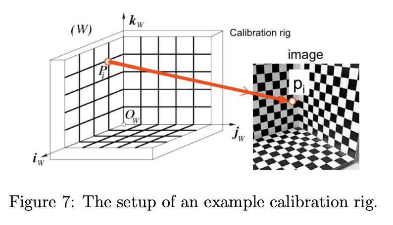
내외부 파라미터를 알고 있으면 실제 3D world로 변환하는것이 가능해진다. 하지만 모든 카메라에 대한 내 외부 파라미터를 알고 있지는 쉽지 않다. 이를 해결하기위해 나온 방법이 camera calibration라는 방법이다. 이는 파라미터들을 추정(estimate)하는 것을 말한다. 아래의 그림에서 보면 이해가 쉬울것이다. 일반적으로 checkerboard를 통해서 일반적인 calibration을 하고 이는 각 코너의 3D 위치를 정확하게 알고 있다. P_{1}, \ldots, P_{n}$를 월드 좌표계로 하고 $p_{1}, \ldots, p_{n}$를 이미지 좌표계로 해서 projection할수 있다.
$P$와 $p$와 camera matrix $M$은 $m_{1}, m_{2}, m_{3}$를 가지고 아래와 같은 수식으로 표현이 되어진다.:
\[p_{i}=\begin{bmatrix} u_{i} \\ v_{i} \end{bmatrix}=M P_{i}=\begin{bmatrix} \frac{m_{1} P_{i}}{m_{3} P_{i}} \\ \frac{m_{2} P_{i}}{m_{3} P_{i}} \end{bmatrix}\]위의 식에서 보듯이, 하나의 대응점(correspondence)은 두 개의 방정식을 제공하며, 따라서 벡터 $m$에 포함된 미지수들을 풀기 위한 두 개의 제약 조건을 제공한다.앞에서는 11개의 partmers가 있고 이를 풀기 위해서는 최소 6개의 대응점이 필요하다. 하지만 노이즈가 많이 생기기 때문에 더 많은 대응점을 사용해야 한다. 노이즈 : 이미지 blur, 렌즈 왜곡, 조명, 센서 노이즈 . 적당하게 20~30개정도가 필요함.
한개의 포인트는 아래와 같은 수식으로 표현이 되어진다. $u_{i}$ and $v_{i}$ with $P_{i}$:
\[\begin{aligned} u_{i}\left(m_{3} P_{i}\right)-m_{1} P_{i} &=0 \\ v_{i}\left(m_{3} P_{i}\right)-m_{2} P_{i} &=0 \end{aligned}\]$n$개의 대응점이 있다면 이렇게 아래와 같이 표현이 되어지며
\[\begin{aligned} u_{1}\left(m_{3} P_{1}\right)-m_{1} P_{1} &=0 \\ v_{1}\left(m_{3} P_{1}\right)-m_{2} P_{1} &=0 \\ \vdots & \\ u_{n}\left(m_{3} P_{n}\right)-m_{1} P_{n} &=0 \\ v_{n}\left(m_{3} P_{n}\right)-m_{2} P_{n} &=0 \end{aligned}\]matrix-vector곱으로 표현되어지면 아래와 같이 표현이 되어지게 되어진다.
\[\begin{bmatrix} P_{1}^{T} & 0^{T} & -u_{1} P_{1}^{T} \\ 0^{T} & P_{1}^{T} & -v_{1} P_{1}^{T} \\ & \vdots & \\ P_{n}^{T} & 0^{T} & -u_{n} P_{n}^{T} \\ 0^{T} & P_{n}^{T} & -v_{n} P_{n}^{T} \end{bmatrix}\begin{bmatrix} m_{1}^{T} \\ m_{2}^{T} \\ m_{3}^{T} \end{bmatrix}=\mathbf{P} m=0\]대응점이 많아졌을경우 에서는 어떻게 Parameter를 찾을까 이는 singular value decomposition (SVD)를 사용하면 된다. $P=U D V^{T}$,로 $V$에 대해서 최소화되어지는 $m$에 대해서 뽑을수 있다.
matrix에 $M$에 있는 백터 $m$을 아래와 같은 수식으로 표현이 되어진다.
\[\rho M=\begin{bmatrix} \alpha r_{1}^{T}-\alpha \cot \theta r_{2}^{T}+c_{x} r_{3}^{T} & \alpha t_{x}-\alpha \cot \theta t_{y}+c_{x} t_{z} \\ \frac{\beta}{\sin \theta} r_{2}^{T}+c_{y} r_{3}^{T} & \frac{\beta}{\sin \theta} t_{y}+c_{y} t_{z} \\ r_{3}^{T} & t_{z} \end{bmatrix}\]Here, $r_{1}^{T}, r_{2}^{T}$, and $r_{3}^{T}$ are the three rows of $R$. Dividing by the scaling parameter gives:
\[M=\frac{1}{\rho}\begin{bmatrix} \alpha r_{1}^{T}-\alpha \cot \theta r_{2}^{T}+c_{x} r_{3}^{T} & \alpha t_{x}-\alpha \cot \theta t_{y}+c_{x} t_{z} \\ \frac{\beta}{\sin \theta} r_{2}^{T}+c_{y} r_{3}^{T} & \frac{\beta}{\sin \theta} t_{y}+c_{y} t_{z} \\ r_{3}^{T} & t_{z} \end{bmatrix}=\begin{bmatrix} A & b \end{bmatrix}=\begin{bmatrix} a_{1}^{T} \\ a_{2}^{T} \\ a_{3}^{T} \end{bmatrix}\begin{bmatrix} b_{1} \\ b_{2} \\ b_{3} \end{bmatrix}\]Solving for the intrinsics gives:
\[\begin{aligned} \rho &=\pm \frac{1}{\left\|a_{3}\right\|} \\ c_{x} &=\rho^{2}\left(a_{1} \cdot a_{3}\right) \\ c_{y} &=\rho^{2}\left(a_{2} \cdot a_{3}\right) \\ \theta &=\cos ^{-1}\left(-\frac{\left(a_{1} \times a_{3}\right) \cdot\left(a_{2} \times a_{3}\right)}{\left\|a_{1} \times a_{3}\right\| \cdot\left\|a_{2} \times a_{3}\right\|}\right) \\ \alpha &=\rho^{2}\left\|a_{1} \times a_{3}\right\| \sin \theta \\ \beta &=\rho^{2}\left\|a_{2} \times a_{3}\right\| \sin \theta \end{aligned}\]The extrinsics are:
\[\begin{aligned} r_{1} &=\frac{a_{2} \times a_{3}}{\left\|a_{2} \times a_{3}\right\|} \\ r_{2} &=r_{3} \times r_{1} \\ r_{3} &=\rho a_{3} \\ T &=\rho K^{-1} b \end{aligned}\]6. Handling Distortion in Camera Calibration
종종 왜곡은 렌즈의 물리적 대칭성 때문에 방사 대칭(radially symmetric)을 가진다. 아래와 같이 등방성으로 모델링을 할수 있따
\[Q P_{i}=\begin{bmatrix} \frac{1}{\lambda} & 0 & 0 \\ 0 & \frac{1}{\lambda} & 0 \\ 0 & 0 & 1 \end{bmatrix} M P_{i}=\begin{bmatrix} u_{i} \\ v_{i} \end{bmatrix}=p_{i}\]If we try to rewrite this into a system of equations as before, we get:
\[\begin{aligned} u_{i} q_{3} P_{i} &=q_{1} P_{i} \\ v_{i} q_{3} P_{i} &=q_{2} P_{i} \end{aligned}\]This system, however, is no longer linear, and we require the use of nonlinear optimization techniques. We can simplify the nonlinear optimization of the calibration problem if we make certain assumptions. In radial distortion, we note that the ratio between two coordinates $u_{i}$ and $v_{i}$ is not affected. We can compute this ratio as:
\[\frac{u_{i}}{v_{i}}=\frac{\frac{m_{1} P_{i}}{m_{3} P_{i}}}{\frac{m_{2} P_{i}}{m_{3} P_{i}}}=\frac{m_{1} P_{i}}{m_{2} P_{i}}\]Assuming that $n$ correspondences are available, we can set up the system of linear equations:
\[\begin{gathered} v_{1}\left(m_{1} P_{1}\right)-u_{1}\left(m_{2} P_{1}\right)=0 \\ \vdots \\ v_{n}\left(m_{1} P_{n}\right)-u_{n}\left(m_{2} P_{n}\right)=0 \end{gathered}\]Similar to before, this gives a matrix-vector product that we can solve via SVD:
\[L n=\begin{bmatrix} v_{1} P_{1}^{T} & -u_{1} P_{1}^{T} \\ \vdots & \vdots \\ v_{n} P_{n}^{T} & -u_{n} P_{n}^{T} \end{bmatrix}\begin{bmatrix} m_{1}^{T} \\ m_{2}^{T} \end{bmatrix}\]Once $m_{1}$ and $m_{2}$ are estimated, $m_{3}$ can be expressed as a nonlinear function of $m_{1}, m_{2}$, and $\lambda$. This requires to solve a nonlinear optimization problem whose complexity is much simpler than the original one.